E/R model Enhanced E/R-model (EE/R-model) Relationelle model Relationelle algebra Omformning fra E/R-model til relationelle model Tirsdag.

Præsentationer af emnet: "E/R model Enhanced E/R-model (EE/R-model) Relationelle model Relationelle algebra Omformning fra E/R-model til relationelle model Tirsdag."— Præsentationens transcript:

1 E/R model Enhanced E/R-model (EE/R-model) Relationelle model Relationelle algebra Omformning fra E/R-model til relationelle model Tirsdag

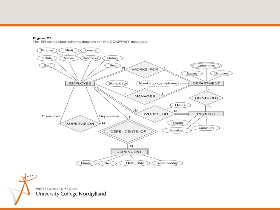
2 ER Diagram for the Company Database

3 EE/R-diagram

4 Den relationelle model Den relationelle model er en datamodel med specielt sigte på relationsdatabaser Den relationelle model er en logisk datamodel, der beskriver hvordan data struktureres i relationsdatabaser

5 Den relationelle model Den relationelle model beskrives ved hjælp af en række veldefinerede begreber: domæner relationelle skemaer relationer attributter tupler primærnøgler, fremmednøgler begrænsninger (constraints)

6 Eksempel på tabeller som repræsentation af relationer

7 Den relationelle model Data struktureres i et antal tabeller (relationer), som har forskellige navne. Hver tabel består af et antal (>=1) søjler (attributter). Attributter er atomiske og defineret over et domæne. I en tabel er der et antal (evt. ingen) rækker (forekomster, tupler), som ikke har nogen indbyrdes orden De enkelte forekomster kan identificeres ved hjælp af værdien af nøglen, der findes ikke to helt ens forekomster En relation (tabel) er en mængde af tupler Graden af en tabel angiver antal attributter (søjler)

8 Nøglebegrebet En nøgle er en attributkombination, som entydigt identificerer en forekomst i en tabel. En nøgle er minimal, dvs.. fjernes een attribut, er den ikke længere entydig. Alle attributter fra tabellen vil tilsammen altid være en (evt.. ikke-minimal) nøgle, kaldet en supernøgle. Der kan være flere forskellige kandidatnøgler i en tabel Der vælges altid en primærnøgle fra mængden af kandidatnøgler

9 Tabelsammenhænge repræsenteres ved fremmednøgler en fremmednøgle er een eller flere attributter i en tabel, som svarer til primærnøglen i en anden tabel en fremmednøgle peger på en forekomst i en anden tabel og fortæller, at her ligger resten af oplysningerne fremmednøglen og primærnøgleattributterne i den tabel, der refereres til, skal have samme domæne.

10 Integritetsregler Integritet: at være sammenhængende Domæneregel: Værdien af en attribut skal være en atomisk værdi fra dom(A) Entitetsintegritet: En primærnøgle må ikke indeholde NULL-værdier Referenceintegritet: En fremmednøgle skal enten være NULL eller referere til en forekomst med en tilsvarende primærnøgleværdi Semantisk integritet: Forskellige regler, der i modsætning til de andre former for integritet, afhænger af den bestemte database.

11 Eksempel I firmaet Minibank registreres der oplysninger om kunder og konti. Om kunder registreres navn, adresse, cprnr og status (A= særlig gode kunder, B= almindelige kunder eller C= problemkunder). Om konti registreres kontonr, saldo og rentefod. En konto hører altid til en og kun en kunde, en kunde kan have 0 eller flere konti. Model: Kunde Konto n 1

12 Eksempel...-2 Der er defineres tre tabeller Kunde Konto PNrBy (for at undgå redundans) For at repræsentere ejerforholdet mellem konto og kunde tilføjes cprnr til konto som fremmednøgle

13 Eksempel …-3 Vi får følgende relationelle skemaer: Kunde: cprnr:cprNrTypePK navnvarChar gadevarChar postnrchar[4]FKREF PNrBy(pnr) statusstatusTypeNOT NULL PNrBy: pnrchar[4]PK byvarCharNOT NULL

14 Eksempel…-4 Konto: ktoktoNrTypePK saldodecimal[>=0]NOT NULL rentefodinterval[0:100]NOT NULL kCprnrcprNrTypeNOT NULL FK REF Kunde(cprnr)

15 Eksempel…-5 domæner: cprNrType: det skal være muligt at definere gyldige cpr-numre (mulige datoer, modulus 11) tilsvarende for kontonumre og statusværdier saldo skal være ikke-negativ (semantisk/problemspecifik) entitet: primærnøgler må ikke være NULL reference: hvad skal der ske med Konto.kCprNr, hvis kunde slettes? ( NULLIFY eller CASCADE) hvad skal der ske med Kunde.postnr, hvis en by får nyt postnr?

16 Semantiske (Problemspecifikke) integritetsregler (forretningsregler) Mulighed for at definere fornuftige reaktioner på forsøg på opdateringer, som vil bryde integritetsregler fx. at hæve et beløb, så saldo vil blive negativ

17 DBMS-understøttelse DBMS’et bør understøtte: 1.Domæneintegritet 2.Entitetsintegritet 3.Referenceintegritet 4.Semantisk integritet Udbredte relationelle DBMS understøtter kun 1 og 4 i begrænset omfang.

18 5.5

19 5.6

20 Foreign Key Constraints

21 Øvelser - papir Opgave 5.11 - s.162

22 Relationel algebra

23 Datamanipulation i den relationelle model - relationsalgebraen Arbejder på hele tabeller dvs. alle operationer tager tabeller som input og returnerer nye tabeller Hermed kan operationer sammensættes til udtryk (som almindelige regneudtryk) Operationer: rækkeudvælgelse (RESTRICT/SELECT) søjleudvælgelse (PROJECT) sammensætning af tabeller (JOIN) mængdeoperationer (UNION, INTERSECTION, MINUS, PRODUCT) avancerede operationer (OUTER (LEFT/RIGTH) JOIN) Det er det, man forstår ved en algebra!

24 Unary Relational Operations SELECT Operation SELECT operation is used to select a subset of the tuples from a relation that satisfy a selection condition. It is a filter that keeps only those tuples that satisfy a qualifying condition – those satisfying the condition are selected while others are discarded. Example: To select the EMPLOYEE tuples whose department number is four or those whose salary is greater than $30,000 the following notation is used:  DNO = 4 (EMPLOYEE)  SALARY > 30,000 (EMPLOYEE) In general, the select operation is denoted by  (R) where the symbol  (sigma) is used to denote the select operator, and the selection condition is a Boolean expression specified on the attributes of relation R

25 Unary Relational Operations SELECT Operation Properties The SELECT operation   (R) produces a relation S that has the same schema as R The SELECT operation  is commutative; i.e.,   (   ( R)) =   (   ( R)) A cascaded SELECT operation may be applied in any order; i.e.,   (   (   ( R))  =   (   (   ( R))) A cascaded SELECT operation may be replaced by a single selection with a conjunction of all the conditions; i.e.,   (   (   ( R))  =   AND AND ( R)))

26 Unary Relational Operations (cont.) Figur 6.1

27 Unary Relational Operations (cont.) PROJECT Operation This operation selects certain columns from the table and discards the other columns. The PROJECT creates a vertical partitioning – one with the needed columns (attributes) containing results of the operation and other containing the discarded Columns. Example: To list each employee’s first and last name and salary, the following is used:   LNAME, FNAME,SALARY (EMPLOYEE) The general form of the project operation is  (R) where  (pi) is the symbol used to represent the project operation and is the desired list of attributes from the attributes of relation R. The project operation removes any duplicate tuples, so the result of the project operation is a set of tuples and hence a valid relation.

28 Unary Relational Operations (cont.) PROJECT Operation Properties The number of tuples in the result of projection   R  is always less or equal to the number of tuples in R. If the list of attributes includes a key of R, then the number of tuples is equal to the number of tuples in R.     R  )    R  as long as   contains the  attributes in 

29 Unary Relational Operations (cont.) Figur 6.1

30 Relational Algebra Operations From Set Theory UNION Example STUDENT U INSTRUCTOR

31 Relational Algebra Operations From Set Theory (cont.) INTERSECTION OPERATION The result of this operation, denoted by R  S, is a relation that includes all tuples that are in both R and S. The two operands must be "type compatible" Example: The result of the intersection operation (figure below) includes only those who are both students and instructors. STUDENT   INSTRUCTOR

32 Relational Algebra Operations From Set Theory (cont.) Set Difference (or MINUS) Operation The result of this operation, denoted by R - S, is a relation that includes all tuples that are in R but not in S. The two operands must be "type compatible”. Example: The figure shows the names of students who are not instructors, and the names of instructors who are not students. STUDENT-INSTRUCTOR INSTRUCTOR- STUDENT

33 Relational Algebra Operations From Set Theory (cont.) Notice that both union and intersection are commutative operations; that is R  S = S  R, and R  S = S  R Both union and intersection can be treated as n-ary operations applicable to any number of relations as both are associative operations; that is R  (S  T) = (R  S)  T, and (R  S)  T = R  (S  T) The minus operation is not commutative; that is, in general R - S ≠ S – R

34 Relational Algebra Operations From Set Theory (cont.) Figur 6.5

35 Binary Relational Operations JOIN Operation The sequence of cartesian product followed by select is used quite commonly to identify and select related tuples from two relations, a special operation, called JOIN. It is denoted by a This operation is very important for any relational database with more than a single relation, because it allows us to process relationships among relations. The general form of a join operation on two relations R(A 1, A 2,..., A n ) and S(B 1, B 2,..., B m ) is: R S where R and S can be any relations that result from general relational algebra expressions.

36 Binary Relational Operations (cont.) Example: Suppose that we want to retrieve the name of the manager of each department. To get the manager’s name, we need to combine each DEPARTMENT tuple with the EMPLOYEE tuple whose SSN value matches the MGRSSN value in the department tuple. We do this by using the join operation. DEPT_MGR  DEPARTMENT MGRSSN=SSN EMPLOYEE

37 Binary Relational Operations (cont.) EQUIJOIN Operation The most common use of join involves join conditions with equality comparisons only. Such a join, where the only comparison operator used is =, is called an EQUIJOIN. In the result of an EQUIJOIN we always have one or more pairs of attributes (whose names need not be identical) that have identical values in every tuple. The JOIN seen in the previous example was EQUIJOIN. NATURAL JOIN Operation Because one of each pair of attributes with identical values is superfluous, a new operation called natural join—denoted by *—was created to get rid of the second (superfluous) attribute in an EQUIJOIN condition. The standard definition of natural join requires that the two join attributes, or each pair of corresponding join attributes, have the same name in both relations. If this is not the case, a renaming operation is applied first.

38 Binary Relational Operations (cont.) EQUIJOIN Operation The most common use of join involves join conditions with equality comparisons only. Such a join, where the only comparison operator used is =, is called an EQUIJOIN. In the result of an EQUIJOIN we always have one or more pairs of attributes (whose names need not be identical) that have identical values in every tuple. The JOIN seen in the previous example was EQUIJOIN. NATURAL JOIN Operation Because one of each pair of attributes with identical values is superfluous, a new operation called natural join—denoted by *—was created to get rid of the second (superfluous) attribute in an EQUIJOIN condition. The standard definition of natural join requires that the two join attributes, or each pair of corresponding join attributes, have the same name in both relations. If this is not the case, a renaming operation is applied first.

39 Binary Relational Operations (cont.) Example: To apply a natural join on the DNUMBER attributes of DEPARTMENT and DEPT_LOCATIONS, it is sufficient to write: (B) DEPT_LOCS  DEPARTMENT * DEPT_LOCATIONS

40 Recap of Relational Algebra Operations

41 Additional Relational Operations Aggregate Functions and Grouping A type of request that cannot be expressed in the basic relational algebra is to specify mathematical aggregate functions on collections of values from the database. Examples of such functions include retrieving the average or total salary of all employees or the total number of employee tuples. These functions are used in simple statistical queries that summarize information from the database tuples. Common functions applied to collections of numeric values include SUM, AVERAGE, MAXIMUM, and MINIMUM. The COUNT function is used for counting tuples or values.

42 Additional Relational Operations (cont.)

43 Use of the Functional operator ℱ ℱ MAX Salary (Employee) retrieves the maximum salary value from the Employee relation ℱ MIN Salary (Employee) retrieves the minimum Salary value from the Employee relation ℱ SUM Salary (Employee) retrieves the sum of the Salary from the Employee relation DNO ℱ COUNT SSN, AVERAGE Salary (Employee) groups employees by DNO (department number) and computes the count of employees and average salary per department.[ Note: count just counts the number of rows, without removing duplicates] Additional Relational Operations (cont.)

44 In NATURAL JOIN tuples without a matching (or related) tuple are eliminated from the join result. Tuples with null in the join attributes are also eliminated. This amounts to loss of information. A set of operations, called outer joins, can be used when we want to keep all the tuples in R, or all those in S, or all those in both relations in the result of the join, regardless of whether or not they have matching tuples in the other relation. The left outer join operation keeps every tuple in the first or left relation R in R S; if no matching tuple is found in S, then the attributes of S in the join result are filled or “padded” with null values. A similar operation, right outer join, keeps every tuple in the second or right relation S in the result of R S. A third operation, full outer join, denoted by keeps all tuples in both the left and the right relations when no matching tuples are found, padding them with null values as needed. The OUTER JOIN Operation

45 Additional Relational Operations (cont.)

46 Øvelser - papir 6.16 a, b, c,d

47 Relational Algebra - Overview

48 Design Guidelines Normalisation Table Design

49 Informal Design Guidelines Table Semantics A table should hold information about one and only one entity/concept from the real world Don’t mix information about more things in one table Avoid Redundant Information Waste of storage Update Anomalies Minimise NULL-values Storage requirements Multiple interpretations (ambiguity) Disallowing the generation of spurious tuples when joining tables.

50 Semantics Consider this table part of a system to handle loans from a library: Loan: [title, matNo, lno, lname, laddress, date, status] Information about different things in the same table

51 Minimise NULL-values If NULL is the most common value for an attribute, then that attribute may not belong in the table. One out of ten employees has a company car. One out of ten cars are assigned to certain employee. On which side should the foreign key be included? Car Employee 1 1

52 Spurious Tuples Again consider this table part of system to handle loans from a library: Loaner:[lNo, fname, lname,…….] Copy:[matNo,…, lname, …] The relationship between Loaner and Copy is designed by including the loaner’s last name in Copy When Loaner and Copy are joined over lname spurious tuples probably will be generated since lname hardly is unique. For instance ’117 Joe Smith’ will be associated with all copies borrowed by someone with last name ‘Smith’, and all other Smiths will be associated with copies borrowed by Joe. The problem arises when relations are represented by anything else than primary – foreign keys

53 Normalisation Normal forms are the formal way to state design guidelines. Normalisation is the process. 6 normal forms (NF) are defined: 1st, 2nd, 3rd, and Boyce-Codd (BCNF). 4th and 5th NF BCNF is the one of most practical interest.

54 First Normal Form (1NF) A table is on 1NF if All attributes are atomic 1NF has become part of the definition of a relation in the relational model and is achieved trivially.

55 Functional Dependencies the foundation of 2NF, 3NF and BCNF Y is functional dependent (FD) of X, if there for any given value of X always is the same value for Y ( X and Y being any set of attributes). FD is written X -> Y Y is FD of X or X is determinant for Y If X is a candidate key, then X -> Y for all sets of attributes Y. X -> Y implies nothing about Y -> X. Classic example: in an address city is FD of postalCode (or postalCode determines city).

56 A Side Often in literature functional dependencies and normal forms are described using a lot of math and it may seem quite theoretical and complicated BUT FDs are business rules and normal forms are common sense constraints on table design The theory and the math are very useful building tools

57 Second Normal Form (2NF) Is about partial FDs A FD X->Y is a full functional dependency (FFD), if no attribute can be removed from X without also removing the FD X->Y. A FD that is not FFD is called partial. A table is on 2NF if: It is on 1NF All non-key attributes are FFD of all candidate keys. Example: Loan: [title, matNo, lno, lname, laddress, date, status]

58 Third Normal Form (3NF) Is about transitive FDs A FD ( X->Y ) is transitive, if there exists a set of attributes Z satisfying X -> Z and Z -> Y. A table is on 3NF if: It is on 2NF No non-key attribute is transitively dependent of a candidate key. ”postalCode - city”-problem!

59 Transitive FD Ssn  Dmgr_ssn since Ssn  Dnumber and Dnumber  Dmgr_ssn Dnumber is not a key or part of a candidate key for EMP_DEPT

60 Boyce-Codd Normal Form If a table is on BCNF, then it is also on 1., 2. and 3. NF. A table is on BCNF, if all determinants are candidate keys. That is: only candidate key may determine the value of other attributes

61 The Difference between 3NF and BCNF For a table to be on 3NF and not on BCNF it must satisfy: It has more than one candidate key, and The candidate keys are overlapping, that is: they have common attributes. For example:A: [a, b, c, d] candidate keys: (a, b) and (a, d) overlap

62 Guideline for Normalisation All attributes are to depend on the key, the whole key, and nothing but the key. So help me Codd.

63 Transformation from ER Diagram to Relational Schemas Design of Relational Tables

64

65 Table Design Transformation from E/R-model to Relational Model Eigth Steps Algorithm Does not always yield an optimal design, but provides a good starting point for the final design of tables

66 Step 1: For each regular entity create a table For composite attributes only the components are included. Multi-value attributes are not included (they are considered in step 6). Choose a primary key.

67 Step 2: For each weak entity type create a table All attributes from the weak entity are included. The primary key from the owner is included as foreign key. The primary key is composed by the owner’s primary key and the partial key.

68 Any attribute on the relation type is included with the key. If possible, include on a side with total participation. Step 3: For each (binary) 1:1-relation type include primary key of one participant as foreign key in the other

69 Any attribute is included with the key on the n-side. Step 4: For each (binary) 1:n relation type include primary key of 1- side as foreign key on n-side

70 Any attribute on the relation is included in the new table. Primary key is composed of the foreign keys. This may also be applied to binary 1:1- and 1:n relations – in particularly if there are relatively few instants of the relation type. Step 5: For each (binary) n:m relation type create table with participating entity types primary keys as foreign keys

71 The primary key of the new table is composed of the foreign key and the multi value attribute. Step 6: For each multi value attribute create table with primary key of entity type as foreign key and the multi value attribute

72 Step 7: For each n-ary (n>2) relation type create a table with the primary keys of all participating entity types as foreign keys Any attribute on the relation type is included. The primary key is composed of the included foreign keys.

73 Result

74 A. The General (the ”nice”) way Create a table for the super class and one for each subclass. In the table for the super class one may add a type attribute. In the tables for the subclasses the primary key from the super class is included and used as primary key. Step 8: Choose one of the following

75 B. Pull-down (only in case of disjoint, total specialisation): Create a table for each subclass Include (“pull down”) all attributes from the super class in each table Use the primary key from the super class as primary key in the new tables Step 8:

76 C. Pull-up-1: (only in case of disjoint specialisation): Create one table for the superclass Include (pull up) all attributes from the subclasses Add a type attribute

77 D. Pull-up-2: (in case of overlapping specialisation): Create one table for the superclass Include (pull up) all attributes from the subclasses Add a type flag for each subclass Step 8 :

78 Table Design Discussion: A: may always be applied, conserves the conceptual model best, may be expensive in joins. B: is only to be applied in case of a disjoint and total specialisation. Saves joins. In case of a partial specialisation entities which are not member of any subclass disappears In the case of overlapping specialisations redundancy is generated C: may be applied in the case of disjoint specialisation. Saves joins Is only to be consider if there are few attributes in the subclasses, since NULL-values are generated D: may be applied instead of C in the case of an overlapping specialisation. The same remarks as for C applies